Modelling Dynamic Operating Envelopes with Gridcognition

Distribution limits

Australia is leading the world on the deployment of distributed generation and South Australia is the poster child for this; we had events last year where almost all of SA’s electrical load was met by roof-top solar.

But there is a limit to how much roof-top solar our local distribution networks can host safely. Increasingly Distribution Network Service Providers (DNSPs) are setting fixed exports limits when customers are requesting to connect new distributed generation systems. These limits are inherently very conservative because they are generally set at the time of connection and have to account for the potential state of the network at all times.

One way of viewing the situation is that we have a market for electricity (imagine your local farmers market), but because of the limits of the distribution network (imagine congested single-lane roads), the owners of distributed energy resources (DERs) can’t get their energy to market (imagine lots of ripe green electrons withering on the vine). The ‘withering on the vine’ in our metaphor represents unnecessary solar curtailment.

DNSPs could invest in more distribution network capacity (bigger roads) to enable more local generation, say from solar PV. This is expensive, and there is question of economic efficiency: is the cost of augmenting the network less than the market value of curtailed generation. This also risks shifting increased network costs onto other network users who may not have the benefit of their own distributed generation system (something new “sun tax” regulations are seeking to address).

A problem with traditional fixed export (and import) limits is that they apply at all times of the day or year, irrespective of the current state of the network. While there may be no capacity to export any energy at a particular connection point in the middle of the day, or perhaps no capacity in the middle of the day in Spring and Autumn, there could be lots of capacity to safely enable exports at other times.

Enter Dynamic Operating Envelopes

The goal of ‘Dynamic Operating Envelopes’ (DOE) is to accurately and dynamically determine the safe operating limits, or the safe upper and lower bounds for imports and exports, and to publish these limits to the distributed energy resources (DERs) connected to the network. This needs to be done in a principled way such that the network’s capacity is shared out fairly to all network users.

Gridcognition

Our mission is to help accelerate the deployment of clean distributed energy systems. We do this with software to support up-front project modelling and ongoing asset performance management.

Using Gridcognition you can model your DER projects before your investment decision, considering options like site selection, asset selection and sizing, asset controls and optimisation, and commercial model, and also considering how network constraints could change your project’s economics.

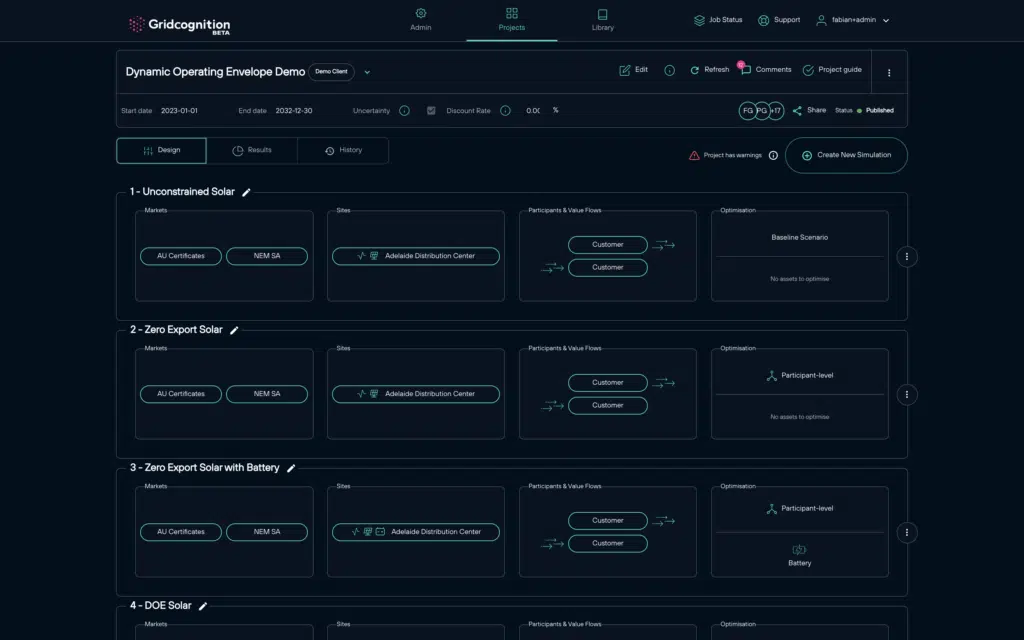
To explore the idea of Dynamic Operating Envelopes I created a very simple project model for a large Warehouse Distribution Center with a 2MW roof-top solar PV system. I then compared four scenarios:

1. Zero export limit
2. Dynamic operating envelope
3. Zero export limit with addition of a battery
4. Dynamic operating envelope with addition of a battery

These are all compared against a baseline scenario where there is unconstrained network access. This is obviously a very hypothetical example, but it demonstrates some interesting points, and shows how Dynamic Operating Envelopes can be reflected in project models.

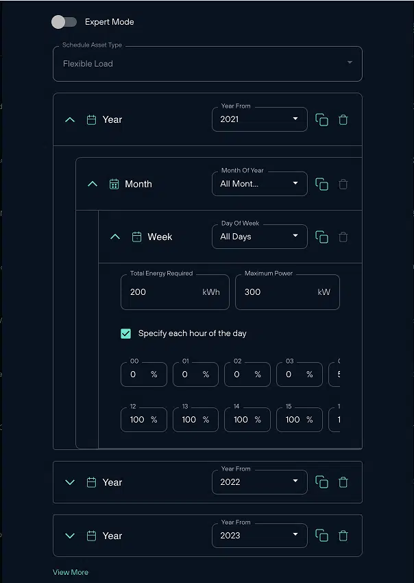
We can define Dynamic Operating Envelopes using ‘Schedules’ in Gridcognition.

Schedules are a very powerful and flexible Gridcognition feature than can be used in a variety of different ways in your projects. Schedules represent a way of describing utilisation or flexibility requirements and are most often used in Gridcognition to support electric vehicle charging models and flexible loads.

You can create your own Schedules in the Gridcognition Library by setting the date (year, month, and day of week) and energy parameters (power or energy requirements/limits), as illustrated to the right. This allows for schedules that vary over years (like increasing EV charger utilisation in future years), vary seasonally (like reflecting times of year when there is more peak demand capacity on a distribution network), and vary by day of week (like reflecting more flexibility to turn down a boiler on Sundays than on Mondays).

When data formats emerge for publishing Dynamic Operating Envelopes we will support uploading these into project models, in the same way Gridcognition supports, for example, uploading interval meter data in NEM12 file format. And if and when DNSPs provide data services (APIs) to publish Dynamic Operating Envelopes we will integrate with these, in the same way Gridcognition integrates with data services provided by market operators to enable access to market settlement data in project models.

For the purposes of this simple project model I defined a very simple Schedule with zero export between 9:00am and 4:00pm and unconstrained import.

Static vs. Dynamic

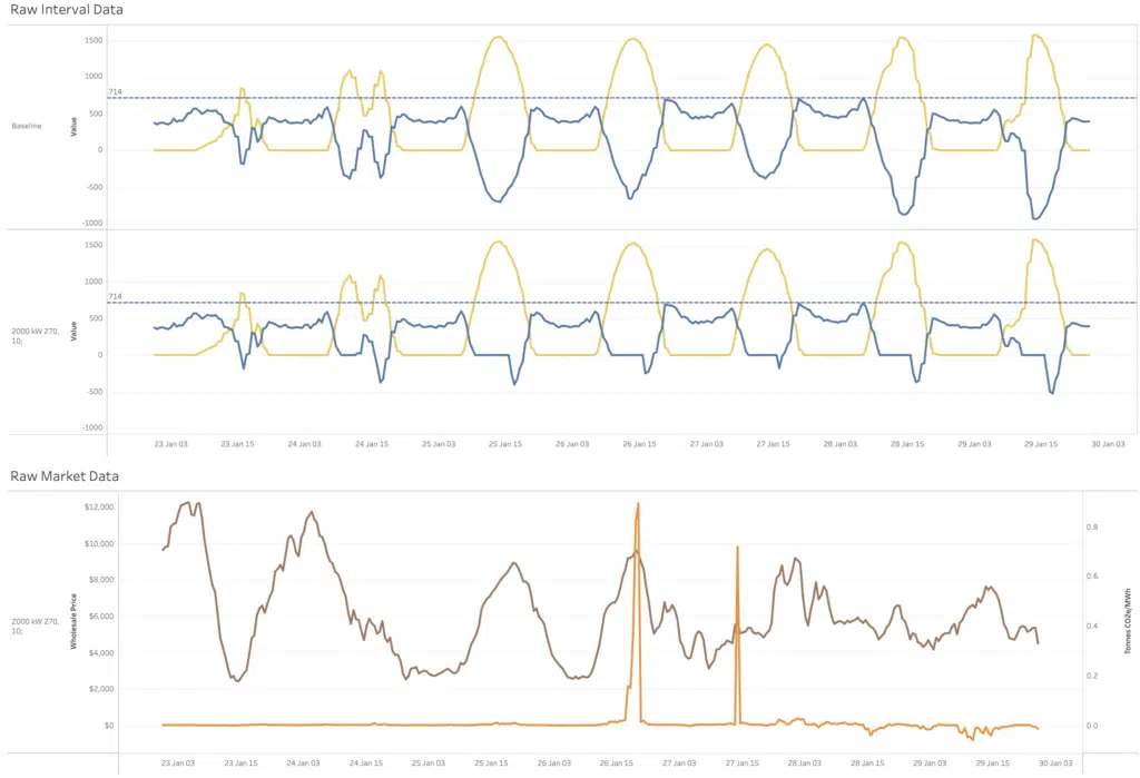
We can use Gridcognition to see the energy generated and exported at an interval level.

Figure 1 below shows a snapshot of a week with our unconstrained baseline scenario in the interval chart above, and our zero export limit in the interval chart below.

This is presented with a third chart showing wholesale market prices, noting some interesting high price events, and interval level grid emissions, showing that ‘middle-of-the-day’ emissions when solar exports are being curtailed are often relatively low.

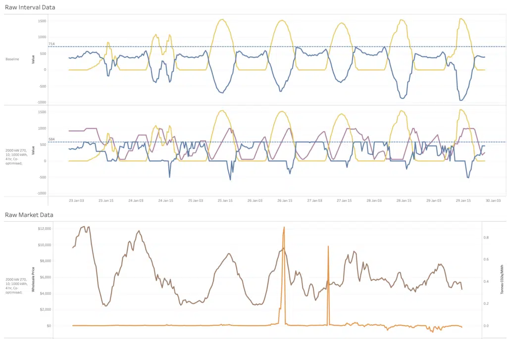
We can contrast this with our Dynamic Operating Envelope scenario, in Figure 2 below. While we still have significant curtailment of exports, we are seeing some excess renewable energy being made available to other energy users.

Battery dynamics

What happens when we add a Battery Energy Storage System to these scenarios?

The static limit with zero-export is shown first. The purple trace on the interval chart below shows the state-of-charge of the 1MWh BESS we have added to the site. The battery is flattening out demand at the site (responding to a network demand charge) and is maximising the self-consumption of solar PV energy.

In our Dynamic Operating Envelope scenario we are seeing more of the batteries capacity being used to export energy to the network, at the expense of a slightly higher maximum demand at the site. This is because the site now has access to the Wholesale Energy Market as an additional value stream the battery can optimise for. However, this effect isn’t dramatic because there isn’t enough value to using the capacity of the battery just for load shifting to maximise wholesale value because of the relatively high benefit of mitigating network demand charges.

Project economics

We don’t just have to peer at interval profiles. We can also look at how static and dynamic operating envelopes impact on project economics.

To keep this model simple, we have assumed our Customer owns the Roof-top Solar PV system and is directly participating in the Wholesale Energy Market.

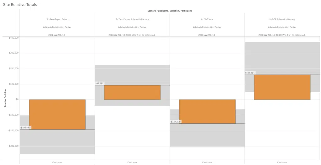
The chart below shows the relative loss of wholesale energy value over a 10-year project duration compared to a baseline with unconstrained network access. That is, our zero-export limit costs our customer $192k, where as our dynamic operating envelope reduces this to a loss of revenue to ‘only’ $152k.

What happens when we add the battery to the project model? In this case the relative cashflows become more complex. Not only are we impacting wholesale energy value (orange), we are also impacting environmental certificate value (green), reducing network costs (red), gaining potential access to the FCAS market (purple), and we have the capex and open associated with our battery to recover (teal).

The bottom line is that while our battery does create value, it doesn’t create enough in this case to offset the capex and opex costs, for this project at least.

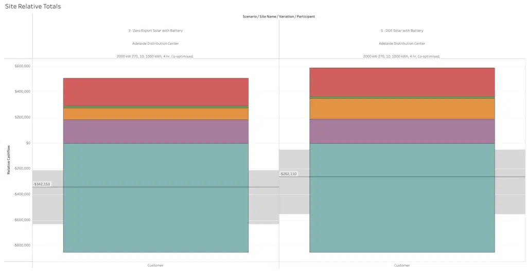
But when we focus just on wholesale energy value, we do see an interesting story. Relative to our solar-PV-only baseline with unconstrained network access, our battery has created $92k of wholesale energy value with the zero export limit, and $159k of wholesale energy value with our dynamic operating limit.

Concluding thoughts

Dynamic Operating Envelopes are a promising way to enable more distributed energy resources to be integrated into the power grid, and, relative to static network limits, they can create significant value for the owners of these resources. While it is early days for this concept, using Gridcognition you can test your projects against different project scenarios including different distribution network limits, helping to make your project more bankable and secure.